where \(F\) is the amount of heat conducted across a unit
cross-sectional area in unit time (W m-2),
\(\lambda\) is thermal conductivity (W m-1
K-1), and \(\nabla T\) is the spatial gradient of
temperature (K m-1). In one-dimensional form
where \(z\) is in the vertical direction (m) and is positive
downward and \(F_{z}\) is positive upward. To account for
non-steady or transient conditions, the principle of energy conservation
in the form of the continuity equation is invoked as
where \(c\) is the volumetric snow/soil heat capacity (J
m-3 K-1) and \(t\) is time (s).
Combining equations and yields the second law of heat conduction in
one-dimensional form
This equation is solved numerically to calculate the soil, snow, and
surface water temperatures for a 25-layer soil column with up to
twelve overlying layers of snow and a single surface water layer with the
boundary conditions of \(h\) as the heat flux into the top soil,
snow, and surface water layers from the overlying atmosphere (section
2.6.1) and zero heat flux at the bottom
of the soil column. The temperature profile is calculated first without
phase change and then readjusted for phase change (section 2.6.2).
The soil column is discretized into 25 layers (section
2.2.2) where \(N_{levgrnd} = 25\) is the
number of soil layers (Table 2.2.3).
The overlying snow pack is modeled with up to twelve layers depending on
the total snow depth. The layers from top to bottom are indexed in the
Fortran code as \(i=-4,-3,-2,-1,0\), which permits the accumulation
or ablation of snow at the top of the snow pack without renumbering the
layers. Layer \(i=0\) is the snow layer next to the soil surface and
layer \(i=snl+1\) is the top layer, where the variable \(snl\)
is the negative of the number of snow layers. The number of snow layers
and the thickness of each layer is a function of snow depth
\(z_{sno}\) (m) as follows.
The node depths, which are located at the midpoint of the snow layers,
and the layer interfaces are both referenced from the soil surface and
are defined as negative values
Note that \(z_{h,\, 0}\) , the interface between the bottom snow
layer and the top soil layer, is zero. Thermal properties (i.e.,
temperature \(T_{i}\) [K]; thermal conductivity
\(\lambda _{i}\) [W m-1 K-1];
volumetric heat capacity \(c_{i}\) [J m-3
K-1]) are defined for soil layers at the node depths
(Figure 2.6.1) and for snow layers at the layer midpoints. When present,
snow occupies a fraction of a grid cell’s area, therefore snow depth
represents the thickness of the snowpack averaged over only the snow
covered area. The grid cell average snow depth is related to the depth
of the snow covered area as \(\bar{z}_{sno} =f_{sno} z_{sno}\) . By
default, the grid cell average snow depth is written to the history
file.
The heat flux \(F_{i}\) (W m-2) from layer \(i\)
to layer \(i+1\) is
These equations are derived, with reference to
Figure 2.6.1, assuming
that the heat flux from \(i\) (depth \(z_{i}\) ) to the
interface between \(i\) and \(i+1\) (depth \(z_{h,\, i}\) )
equals the heat flux from the interface to \(i+1\) (depth
\(z_{i+1}\) ), i.e.,
where \(T_{m}\) is the temperature at the interface of layers
\(i\) and \(i+1\).
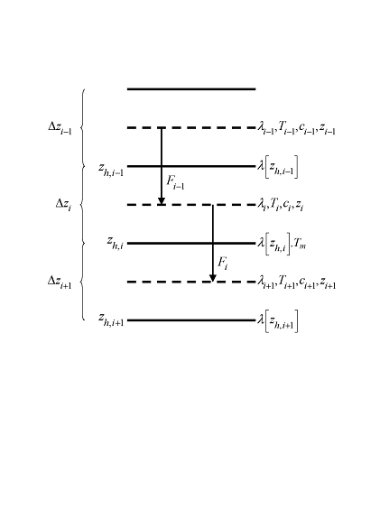
Shown are three soil layers, \(i-1\), \(i\), and \(i+1\).
The thermal conductivity \(\lambda\) , specific heat capacity
\(c\), and temperature \(T\) are defined at the layer node depth
\(z\). \(T_{m}\) is the interface temperature. The thermal
conductivity \(\lambda \left[z_{h} \right]\) is defined at the
interface of two layers
\(z_{h}\) . The layer thickness is \(\Delta z\). The heat fluxes
\(F_{i-1}\) and \(F_{i}\) are defined as positive upwards.
Figure 2.6.1 Schematic diagram of numerical scheme used to solve for soil temperature.
where the superscripts \(n\) and \(n+1\) indicate values at the
beginning and end of the time step, respectively, and \(\Delta t\)
is the time step (s). This equation is solved using the Crank-Nicholson
method, which combines the explicit method with fluxes evaluated at
\(n\) (\(F_{i-1}^{n} ,F_{i}^{n}\) ) and the implicit method with
fluxes evaluated at \(n+1\) (\(F_{i-1}^{n+1} ,F_{i}^{n+1}\) )
where \(a_{i}\) , \(b_{i}\) , and \(c_{i}\) are the
subdiagonal, diagonal, and superdiagonal elements in the tridiagonal
matrix and \(r_{i}\) is a column vector of constants. When surface
water is present, the equation for the top soil layer has an additional
term representing the surface water temperature; this results in a four
element band-diagonal system of equations.
For the top soil layer \(i=1\) , top snow layer \(i=snl+1\), or
surface water layer, the heat flux from the overlying atmosphere
\(h\) (W m-2, defined as positive into the surface)
is
where \(\overrightarrow{S}_{sno}\) is the solar radiation absorbed
by the top snow layer (section 2.3.2.1), \(\overrightarrow{L}_{sno}\)
is the longwave radiation absorbed by the snow (positive toward the
atmosphere) (section 2.4.2), \(H_{sno}\) is the
sensible heat flux from the snow (Chapter
2.5), and
\(\lambda E_{sno}\) is the latent heat flux from the snow (Chapter
2.5). The partial
derivative of the heat flux \(h\) with respect to temperature is
and the partial derivatives of the sensible and latent heat fluxes are
given by equations and for non-vegetated surfaces, and by equations and
for vegetated surfaces. \(\sigma\) is the Stefan-Boltzmann constant
(W m-2 K-4) (Table 2.2.7) and
\(\varepsilon _{g}\) is the ground emissivity (section
2.4.2). For purposes of computing \(h\) and
\(\frac{\partial h}{\partial T_{g} }\) , the term \(\lambda\)
is arbitrarily assumed to be
where \(\lambda _{sub}\) and \(\lambda _{vap}\) are the
latent heat of sublimation and vaporization, respectively (J
kg-1) (Table 2.2.7), and \(w_{liq,\, snl+1}\)
and \(w_{ice,\, snl+1}\) are the liquid water and ice contents of the
top snow/soil layer, respectively (kg m-2)
(Chapter 2.7).
For the top soil layer, \(i=1\), the coefficients are
It can be seen that when no snow is present (\(f_{sno} =0\)), the
expressions for the coefficients of the top soil layer have the same
form as those for the top snow layer.
The surface snow/soil layer temperature computed in this way is the
layer-averaged temperature and hence has somewhat reduced diurnal
amplitude compared with surface temperature. An accurate surface
temperature is provided that compensates for this effect and numerical
error by tuning the heat capacity of the top layer (through adjustment
of the layer thickness) to give an exact match to the analytic solution
for diurnal heating. The top layer thickness for \(i=snl+1\) is
given by
where \(c_{a}\) is a tunable parameter, varying from 0 to 1, and is
taken as 0.34 by comparing the numerical solution with the analytic
solution (Z.-L. Yang 1998, unpublished manuscript).
\(\Delta z_{i*}\) is used in place of \(\Delta z_{i}\) for
\(i=snl+1\) in equations -. The top snow/soil layer temperature
computed in this way is the ground surface temperature
\(T_{g}^{n+1}\) .
The boundary condition at the bottom of the snow/soil column is zero
heat flux, \(F_{i} =0\), resulting in, for \(i=N_{levgrnd}\) ,
where \(T_{i}^{n+1}\) is the soil layer temperature after solution
of the tridiagonal equation set, \(w_{ice,\, i}\) and
\(w_{liq,\, i}\) are the mass of ice and liquid water (kg
m-2) in each snow/soil layer, respectively, and \(T_{f}\)
is the freezing temperature of water (K) (Table 2.2.7).
For the freezing process in soil layers, the concept of supercooled soil
water from Niu and Yang (2006) is adopted. The supercooled
soil water is the liquid water that coexists with ice over a wide range of
temperatures below freezing and is implemented through a freezing point
depression equation
where \(w_{liq,\, \max ,\, i}\) is the maximum liquid water in
layer \(i\) (kg m-2) when the soil temperature
\(T_{i}\) is below the freezing temperature \(T_{f}\) ,
\(L_{f}\) is the latent heat of fusion (J kg-1)
(Table 2.2.7), \(g\) is the gravitational acceleration (m
s-2) (Table 2.2.7), and \(\psi _{sat,\, i}\) and
\(B_{i}\) are the soil texture-dependent saturated matric potential
(mm) and Clapp and Hornberger (1978) exponent
(section 2.7.3).
For the special case when snow is present (snow mass \(W_{sno} >0\))
but there are no explicit snow layers (\(snl=0\)) (i.e., there is
not enough snow present to meet the minimum snow depth requirement of
0.01 m), snow melt will take place for soil layer \(i=1\) if the
soil layer temperature is greater than the freezing temperature
(\(T_{1}^{n+1} >T_{f}\) ).
The rate of phase change is assessed from the energy excess (or deficit)
needed to change \(T_{i}\) to freezing temperature, \(T_{f}\) .
The excess or deficit of energy \(H_{i}\) (W m-2) is
determined as follows
For the special case when snow is present (\(W_{sno} >0\)), there
are no explicit snow layers (\(snl=0\)), and
\(\frac{H_{1} \Delta t}{L_{f} } >0\) (melting), the snow mass
\(W_{sno}\) (kg m-2) is reduced according to
The ice mass, liquid water content, and temperature of the top soil
layer are then determined from (2.6.54), (2.6.57), and (2.6.59)
using the recalculated energy from (2.6.63). Snow melt \(M_{1S}\)
(kg m-2 s-1) and phase change energy \(E_{p,\, 1S}\)
(W m-2) for this special case are
Phase change of surface water takes place when the surface water
temperature, \(T_{h2osfc}\) , becomes less than \(T_{f}\) . The
energy available for freezing is
where \(c_{h2osfc}\) is the volumetric heat capacity of water, and
\(\Delta z_{h2osfc}\) is the depth of the surface water layer. If
\(H_{m} =\frac{H_{h2osfc} \Delta t}{L_{f} } >0\) then \(H_{m}\)
is removed from surface water and added to the snow column as ice
The thermal properties of the soil are assumed to be a weighted combination of
the mineral and organic properties of the soil
(Lawrence and Slater 2008).
The soil layer organic matter fraction \(f_{om,i}\) is
where \(\lambda _{sat,\, i}\) is the saturated thermal
conductivity, \(\lambda _{dry,\, i}\) is the dry thermal
conductivity, \(K_{e,\, i}\) is the Kersten number,
\(S_{r,\, i}\) is the wetness of the soil with respect to
saturation, and \(\lambda _{bedrock} =3\) W m-1
K-1 is the thermal conductivity assumed for the deep
ground layers (typical of saturated granitic rock;
Clauser and Huenges 1995). For glaciers,
where \(\lambda _{liq}\) and \(\lambda _{ice}\) are the
thermal conductivities of liquid water and ice, respectively (Table 2.2.7). The saturated thermal conductivity \(\lambda _{sat,\, i}\) (W
m-1 K-1) depends on the thermal
conductivities of the soil solid, liquid water, and ice constituents
and \(\lambda _{s,om} =0.25\)W m-1
K-1 (Farouki 1981). \(\theta _{sat,\, i}\) is the
volumetric water content at saturation (porosity) (section 2.7.3.1).
where the thermal conductivity of dry mineral soil
\(\lambda _{dry,\min ,i}\) (W m-1
K-1) depends on the bulk density
\(\rho _{d,\, i} =2700\left(1-\theta _{sat,\, i} \right)\) (kg
m-3) as
and \(\lambda _{dry,om} =0.05\) W m-1
K-1 (Farouki 1981) is the dry thermal conductivity of
organic matter. The Kersten number \(K_{e,\, i}\) is a function of
the degree of saturation \(S_{r}\) and phase of water
The volumetric heat capacity \(c_{i}\) (J m-3 K-1) for
soil is from de Vries (1963) and depends on the
heat capacities of the soil solid, liquid water, and ice constituents
where \(C_{liq}\) and \(C_{ice}\) are the specific heat
capacities (J kg-1 K-1) of liquid water
and ice, respectively (Table 2.2.7). The heat capacity of soil solids
\(c_{s,i}\) (J m-3 K-1) is
where \(c_{s,bedrock} =2\times 10^{6}\) J m-3
K-1 is the heat capacity of bedrock and
\(c_{s,om} =2.5\times 10^{6}\) J m-3
K-1 (Farouki 1981) is the heat capacity of organic
matter. For glaciers and snow
For the special case when snow is present (\(W_{sno} >0\)) but
there are no explicit snow layers (\(snl=0\)), the heat capacity of
the top layer is a blend of ice and soil heat capacity