1. Introduction
CMEPS is a NUOPC-compliant mediator which uses ESMF to couple earth grid components in a hub and spoke system.
As a mediator, CMEPS is responsible for transferring field information from one model component to another. This transfer can require one or more operations on the transferred fields, including mapping of fields between component grids, merging of fields between different components and time-averaging of fields over varying coupling periods.
Components share information via import and export states, which are containers for ESMF data types that wrap native model data. The states also contain metadata, which includes physical field names, the underlying grid structure and coordinates, and information on the parallel decomposition of the fields. Note that while CMEPS itself is a mesh based mediator, component models coupled by the CMEPS mediator can be either grid or mesh based.
Each component model using the CMEPS mediator is serviced by a NUOPC-compliant cap. The NUOPC cap is a small software layer between the underlying model code and the mediator. Fields for which the mediator has created a connection between model components are placed in either the import or export state of the component within the NUOPC cap. The information contained within these states is then passed into native model arrays or structures for use by the component model.
Field connections made by the CMEPS mediator between components rely on matching of standard field names. These standard names are defined in a field dictionary. Since CMEPS is a community mediator, these standard names are specific to each application.
1.1. Organization of the CMEPS mediator code
When you check out the code you will files, which can be organized into three groups:
- totally generic components that carry out the mediator functionality such as mapping, merging, restarts and history writes. Included here is a a “fraction” module that determines the fractions of different source model components on every source destination mesh.
- application specific code that determines what fields are exchanged between components and how they are merged and mapped.
- prep phase modules that carry out the mapping and merging from one or more source components to the destination component.
| Generic Code | Application Specific Code | Prep Phase Code |
|---|---|---|
| med.F90 | esmFldsExchange_cesm_mod.F90 | med_phases_prep_atm_mod.F90 |
| esmFlds.F90 | esmFldsExchange_nems_mod.F90 | med_phases_prep_ice_mod.F90 |
| med_map_mod.F90 | esmFldsExchange_hafs_mod.F90 | med_phases_prep_ocn_mod.F90 |
| med_merge_mod.F90 | fd_cesm.yaml | med_phases_prep_glc_mod.F90 |
| med_frac_mod.F90 | fd_nems.yaml | med_phases_prep_lnd_mod.F90 |
| med_internalstate_mod.F90 | fd_hafs.yaml | med_phases_prep_rof_mod.F90 |
| med_methods_mod.F90. | ||
| med_phases_aofluxes_mod.F90 | ||
| med_phases_ocnalb_mod.F90 | ||
| med_phases_history_mod.F90 | ||
| med_phases_restart_mod.F90 | ||
| med_phases_profile_mod.F90 | ||
| med_io_mod.F90 | ||
| med_constants_mod.F90 | ||
| med_kind_mod.F90 | ||
| med_time_mod.F90 | ||
| med_utils_mod.F90 |
Note
Some modules, such as med_phases_prep_ocn.F90 and med_frac_mod.F90 also contain application specific-code blocks.
1.2. Mapping and Merging Primer
This section provides a primer on mapping (interpolation) and merging of gridded coupled fields. Masks, support for partial fractions on grids, weights generation, and fraction weighted mapping and merging all play roles in the conservation and quality of the coupled fields.
A pair of atmosphere and ocean/ice grids can be used to highlight the analysis.
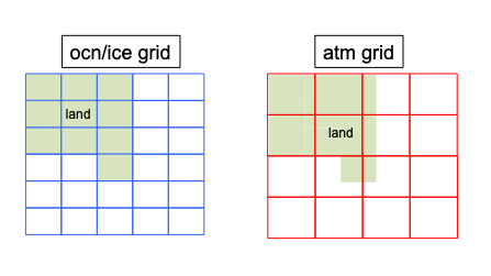
The most general CMEPS mediator assumes the ocean and sea ice surface grids are identical while the atmosphere and land grids are also identical. The ocean/ice grid defines the mask which means each ocean/ice gridcell is either a fully active ocean/ice gridcell or not (i.e. land). Other configurations have been and can be implemented and analyzed as well.
The ocean/ice mask interpolated to the atmosphere/land grid determines the complementary ocean/ice and land masks on the atmosphere grid. The land model supports partially active gridcells such that each atmosphere gridcell may contain a fraction of land, ocean, and sea ice.
Focusing on a single atmosphere grid cell.
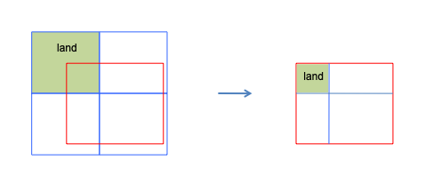
The gridcells can be labeled as follows.
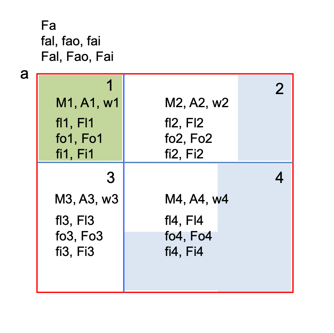
The atmosphere gridcell is labeled “a”. On the atmosphere gridcell (the red box), in general, there is a land fraction (fal), an ocean fraction (fao), and a sea ice fraction (fai). The sum of the surface fractions should always be 1.0 in these conventions. There is also a gridbox average field on the atmosphere grid (Fa). This could be a flux or a state that is derived from the equivalent land (Fal), ocean (Fao), and sea ice (Fai) fields. The gridbox average field is computed by merging the various surfaces:
Fa = fal*Fal + fao*Fao + fai*Fai
This is a standard merge where:
fal + fao + fai = 1.0
and each surface field, Fal, Fao, and Fai are the values of the surface fields on the atmosphere grid.
The ocean gridcells (blue boxes) are labeled 1, 2, 3, and 4 in this example. In general, each ocean/ice gridcell partially overlaps multiple atmosphere gridcells. Each ocean/ice gridcell has an overlapping Area (A) and a Mask (M) associated with it. In this example, land is colored green, ocean blue, and sea ice white so just for the figure depicted:
M1 = 0
M2 = M3 = M4 = 1
Again, the ocean/ice areas (A) are overlapping areas so the sum of the overlapping areas is equal to the atmophere area:
Aa = A1 + A2 + A3 + A4
The mapping weight (w) defined in this example allows a field on the ocean/ice grid to be interpolated to the atmosphere/land grid. The mapping weights can be constructed to be conservative, bilinear, bicubic, or with many other approaches. The main point is that the weights represent a linear sparse matrix such that in general:
Xa = [W] * Xo
where Xa and Xo represent the vector of atmophere and ocean gridcells respectively, and W is the sparse matrix weights linking each ocean gridcell to a set of atmosphere gridcells. Nonlinear interpolation is not yet supported in most coupled systems.
Mapping weights can be defined in a number of ways even beyond conservative or bilinear. They can be masked or normalized using multiple approaches. The weights generation is intricately tied to other aspects of the coupling method. In CMEPS, area-overlap conservative weights are defined as follows:
w1 = A1/Aa
w2 = A2/Aa
w3 = A3/Aa
w4 = A4/Aa
This simple approach which does not include any masking or normalization provides a number of useful attributes. The weights always add up to 1.0:
w1 + w2 + w3 + w4 = 1.0
and a general area weighted average of fields on the ocean/ice grid mapped to the atmosphere grid would be:
Fa = w1*F1 + w2*F2 + w3*F3 + w4*F4
These weights conserve area:
w1*Aa + w2*Aa + w3*Aa + w4*Aa = Aa
and can be used to interpolate the ocean/ice mask to the atmosphere grid to compute the land fraction:
f_ocean = w1*M1 + w2*M2 + w3*M3 + w4*M4
f_land = (1-f_ocean)
These weights also can be used to interpolate surface fractions:
fal = w1*fl1 + w2*fl2 + w3*fl3 + w4*fl4
fao = w1*fo1 + w2*fo2 + w3*fo3 + w4*fo4
fai = w1*fi1 + w2*fi2 + w3*fi3 + w4*fi4
Checking sums:
fal + fao + fai = w1*(fl1+fo1+fi1) + w2*(fl2+fo2+fi2) + w3*(fl3+fo3+fi3) + w4*(fl4+fo4+fi4)
fal + fao + fai = w1 + w2 + w3 + w4 = 1.0
And the equation for f_land and fal above are consistent if fl1=1-M1:
f_land = 1 - f_ocean
f_land = 1 - (w1*M1 + w2*M2 + w3*M3 + w4*M4)

fal = w1*(1-M1) + w2*(1-M2) + w3*(1-M3) + w4*(1-M4)
fal = w1 + w2 + w3 + w4 - (w1*M1 + w2*M2 + w3*M3 + w4*M4)
fal = 1 - (w1*M1 + w2*M2 + w3*M3 + w4*M4)
Clearly defined and consistent weights, areas, fractions, and masks is critical to generating conservation in the system.
When mapping masked or fraction weighted fields, these weights require that the mapped field be normalized by the mapped fraction. Consider a case where sea surface temperature (SST) is to be mapped to the atmosphere grid with:
M1 = 0; M2 = M3 = M4 = 1
w1, w2, w3, w4 are defined as above (ie. A1/Aa, A2/Aa, A3/Aa, A4/Aa)
There are a number of ways to compute the mapped field. The direct weighted average equation, Fa = w1*Fo1 + w2*Fo2 + w3*Fo3 + w4*Fo4, is ill-defined because w1 is non-zero and Fo1 is underfined since it’s a land gridcell on the ocean grid. A masked weighted average, Fa = M1*w1*Fo1 + M2*w2*Fo2 + M3*w3*Fo3 + M4*w4*Fo4 is also problematic because M1 is zero, so the contribution of the first term is zero. But the sum of the remaining weights (M2*w2 + M3*w3 + M4*w4) is now not identically 1 which means the weighted average is incorrect. (To test this, assume all the weights are each 0.25 and all the Fo values are 10 degC, Fa would then be 7.5 degC). Next consider a masked weighted normalized average, f_ocean = (w1*M1 + w2*M2 + w3*M3 + w4*M4) combined with Fa = (M1*w1*Fo1 + M2*w2*Fo2 + M3*w3*Fo3 + M4*w4*Fo4) / (f_ocean) which produces a reasonable but incorrect result because the weighted average uses the mask instead of the fraction. The mask only produces a correct result in cases where there is no sea ice because sea ice impacts the surface fractions. Finally, consider a fraction weighted normalized average using the dynamically varying ocean fraction that is exposed to the atmosphere:
fo1 = 1 - fi1
fo2 = 1 - fi2
fo3 = 1 - fi3
fo4 = 1 - fi4
fao = w1*fo1 + w2*fo2 + w3*fo3 + w4*fo4
Fao = (fo1*w1*Fo1 + fo2*w2*Fo2 + fo3*w3*Fo3 + fo4*w4*Fo4) / (fao)
where fo1, fo2, fo3, and fo4 are the ocean fractions on the ocean gridcells and depend on the sea ice fraction, fao is the mapped ocean fraction on the atmosphere gridcell, and Fa is the mapped SST. The ocean fractions are only defined where the ocean mask is 1, otherwise the ocean and sea ice fractions are zero. Now, the SST in each ocean gridcell is weighted by the fraction of the ocean box exposed to the atmosphere and that weighted average is normalized by the mapped dynamically varying fraction. This produces a reasonable result as well as a conservative result.
The conservation check involves thinking of Fo and Fa as a flux. On the ocean grid, the quantity associated with the flux is:
Qo = (Fo1*fo1*A1 + Fo2*fo2*A2 + Fo3*fo3*A3 + Fo4*fo4*A4) * dt
on the atmosphere grid, that quantity is the ocean fraction times the mapped flux times the area times the timestep:
Qa = foa * Fao * Aa * dt
Via some simple math, it can be shown that Qo = Qa if:
fao = w1*fo1 + w2*fo2 + w3*fo3 + w4*fo4
Fao = (fo1*w1*Fo1 + fo2*w2*Fo2 + fo3*w3*Fo3 + fo4*w4*Fo4) / (fao)
In practice, the fraction weighted normlized mapping field is computed by mapping the ocean fraction and the fraction weighted field from the ocean to the atmosphere grid separately and then using the mapped fraction to normalize the field as a four step process:
Fo' = fo*Fo                                   (a)
fao = w1*fo1 + w2*fo2 + w3*fo3 + w4*fo4       (b)
Fao' = w1*Fo1' + w2*Fo2' + w3*Fo3' + w4*Fo4'  (c)
Fao = Fao'/fao                                (d)
Steps (b) and (c) above are the sparse matrix multiply by the standard conservative weights. Step (a) fraction weighs the field and step (d) normalizes the mapped field.
Another way to think of this is that the mapped flux (Fao’) is normalized by the same fraction (fao) that is used in the merge, so they actually cancel. Both the normalization at the end of the mapping and the fraction weighting in the merge can be skipped and the results should be identical. But then the mediator will carry around Fao’ instead of Fao and that field is far less intuitive as it no longer represents the gridcell average value, but some subarea average value. In addition, that approach is only valid when carrying out full surface merges. If, for instance, the SST is to be interpolated and not merged with anything, the field must be normalized after mapping to be useful.
The same mapping and merging process is valid for the sea ice:
fai = w1*fi1 + w2*fi2 + w3*fi3 + w4*fi4
Fai = (fi1*w1*Fi1 + fi2*w2*Fi2 + fi3*w3*Fi3 + fi4*w4*Fi4) / (fai)
Putting this together with the original merge equation:
Fa = fal*Fal + fao*Fao + fai*Fai
where now:
fal = 1 - (fao+fai)
fao = w1*fo1 + w2*fo2 + w3*fo3 + w4*fo4
fai = w1*fi1 + w2*fi2 + w3*fi3 + w4*fi4
Fal = Fl1 = Fl2 = Fl3 = Fl4 as defined by the land model on the atmosphere grid
Fao = (fo1*w1*Fo1 + fo2*w2*Fo2 + fo3*w3*Fo3 + fo4*w4*Fo4) / (fao)
Fai = (fi1*w1*Fi1 + fi2*w2*Fi2 + fi3*w3*Fi3 + fi4*w4*Fi4) / (fai)
will simplify to an equation that contains twelve distinct terms for each of the four ocean gridboxes and the three different surfaces:
Fa = (w1*fl1*Fl1 + w2*fl2*Fl2  + w3*fl3*Fl3 + w4*fl4*Fl4) +
     (w1*fo1*Fo1 + w2*fo2*Fo2  + w3*fo3*Fo3 + w4*fo4*Fo4) +
     (w1*fi1*Fi1 + w2*fi2*Fi2  + w3*fi3*Fi3 + w4*fi4*Fi4)
and this further simplifies to something that looks like a mapping of the field merged on the ocean grid:
Fa = w1*(fl1*Fl1+fo1*Fo1+fi1*Fi1) +
     w2*(fl2*Fl2+fo2*Fo2+fi2*Fi2) +
     w3*(fl3*Fl3+fo3*Fo3+fi3*Fi3) +
     w4*(fl4*Fl4+fo4*Fo4+fi4*Fi4)
Like the exercise with Fao above, these equations can be shown to be fully conservative.
To summarize, multiple features such as area calculations, weights, masking, normalization, fraction weighting, and merging approaches have to be considered together to ensure conservation. The CMEPS mediator uses unmasked and unnormalized weights and then generally maps using the fraction weighted normalized approach. Merges are carried out with fraction weights. This is applied to both state and flux fields, with conservative, bilinear, and other mapping approaches, and for both merged and unmerged fields. This ensures that the fields are always useful gridcell average values when being coupled or analyzed throughout the coupling implementation.
1.3. Area Corrections
Area corrections are generally necessary when coupling fluxes between different component models if conservation is important. The area corrections adjust the fluxes such that the quantity is conserved between different models. The area corrections are necessary because different model usually compute gridcell areas using different approaches. These approaches are inherently part of the model discretization, they are NOT ad-hoc.
If the previous section, areas and weights were introduced. Those areas were assumed to consist of the area overlaps between gridcells and were computed using a consistent approach such that the areas conserve. ESMF is able to compute these area overlaps and the corresponding mapping weights such that fluxes can be mapped and quantities are conserved.
However, the ESMF areas don’t necessarily agree with the model areas that are inherently computed in the individual component models. As a result, the fluxes need to be corrected by the ratio of the model areas and the ESMF areas. Consider a simple configuration where two grids are identical, the areas computed by ESMF are identical, and all the weights are 1.0. So:
A1 = A2 (from ESMF)
w1 = 1.0 (from ESMF)
F2 = w1*F1  (mapping)
F2*A2 = F1*A1 (conservation)
Now lets assume that the two models have fundamentally different discretizations, different area algorithms (i.e. great circle vs simpler lon/lat approximations), or even different assumptions about the size and shape of the earth. The grids can be identical in terms of the longitude and latitude of the gridcell corners and centers, but the areas can also be different because of the underlying model implementation. When a flux is passed to or from each component, the quantity associated with that flux is proportional to the model area, so:
A1 = A2 (ESMF areas)
w1 = 1.0
F2 = w1*F1 (mapping)
F2 = F1
A1m != A2m  (model areas)
F1*A1m != F2*A2m  (loss of conservation)
This can be corrected by multiplying the fluxes by an area correction. For each model, outgoing fluxes should be multiplied by the model area divided by the ESMF area. Incoming fluxes should be multiplied by the ESMF area divided by the model area. So:
F1' = A1m/A1*F1
F2' = w1*F1'
F2  = F2'*A2/A2m

Q2 = F2*A2m
   = (F2'*A2/A2m)*A2m
   = F2'*A2
   = (w1*F1')*A2
   = w1*(A1m/A1*F1)*A2
   = A1m*F1
   = Q1
and now the mapped flux conserves in the component models. The area corrections should only be applied to fluxes. These area corrections can actually be applied a number of ways.
- The model areas can be passed into ESMF as extra arguments and then the weights will be adjusted. In this case, weights will no longer sum to 1 and different weights will need to be generated for mapping fluxes and states.
- Models can pass quantities instead of fluxes, multiplying the flux in the component by the model area. But this has a significant impact on the overall coupling strategy.
- Models can pass the areas to the mediator and the mediator can multiple fluxes by the source model area before mapping and divide by the destination model area area after mapping.
- Models can pass the areas to the mediator and implement an area correction term on the incoming and outgoing fluxes that is the ratio of the model and ESMF areas. This is the approach shown above and is how CMEPS traditionally implements this feature.
Model areas should be passed to the mediator at initialization so the area corrections can be computed and applied. These area corrections do not vary in time.
1.4. Lags, Accumulation and Averaging
In a coupled model, the component model sequencing and coupling frequency tend to introduce some lags as well as a requirement to accumulate and average. This occurs when component models are running sequentially or concurrently. In general, the component models advance in time separately and the “current time” in each model becomes out of sync during the sequencing loop. This is not unlike how component models take a timestep. It’s generally more important that the coupling be conservative than synchronous.
At any rate, a major concern is conservation and consistency. As a general rule, when multiple timesteps are taken between coupling periods in a component model, the fluxes and states should be averaged over those timesteps before being passed back out to the coupler. In the same way, the fluxes and states passed into the coupler should be averaged over shorter coupling periods for models that are coupled at longer coupling periods.
For conservation of mass and energy, the field that is accumluated should be consistent with the field that would be passed if there were no averaging required. Take for example a case where the ocean model is running at a longer coupling period. The ocean model receives a fraction weighted merged atmosphere/ocean and ice/ocean flux written as:
Fo = fao*Fao + fio*Fio
The averaged flux over multiple time periods, n, would then be:
Fo = 1/n * sum_n(fao*Fao + fio*Fio)
where sum_n represents the sum over n time periods. This can also be written as:
Fo = 1/n * (sum_n(fao*Fao) + sum_n(fio*Fio))
So multiple terms can be summed and accumulated or the individual terms fao*Fao and fio*Fio can be accumulated and later summed and averaged in either order. Both approaches produce identical results. Finally, it’s important to note that sum_n(fao)*sum_n(Fao) does not produce the same results as the sum_n(fao*Fao). In other words, the fraction weighted flux has to be accumulated and NOT the fraction and flux separately. This is important for conservation in flux coupling. The same approach should be taken with merged states to compute the most accurate representation of the average state over the slow coupling period. An analysis and review of each coupling field should be carried out to determine the most conservative and accurate representation of averaged fields. This is particularly important for models like the sea ice model where fields may be undefined at gridcells and timesteps where the ice fraction is zero.
Next, consider how mapping interacts with averaging. A coupled field can be accumulated on the grid where that field is used. As in the example above, the field that would be passed to the ocean model can be accumulated on the ocean grid over fast coupling periods as if the ocean model were called each fast coupling period. If the flux is computed on another grid, it would save computational efforts if the flux were accumulated and averaged on the flux computation grid over fast coupling periods and only mapped to the destination grid on slow coupling periods. Consider just the atmosphere/ocean term above:
1/n * sum_n(fao_o*Fao_o)
which is accumulated and averaged on the ocean grid before being passed to the ocean model. The _o notation has been added to denote the field on on the ocean grid. However, if Fao is computed on the atmosphere grid, then each fast coupling period the following operations would need to be carried out
- Fao_a is computed on the atmosphere grid
- fao_a, the ocean fraction on the atmosphere grid is known
- fao_o = map(fao_a), the fraction is mapped from atmosphere to ocean
- Fao_o = map(Fao_a), the flux is mapped from atmosphere to ocean
- fao_o*Fao_o is accumulated over fast coupling periods
- 1/n * sum_n(fao_o*Fao_o), the accumulation is averaged every slow coupling period
Writing this in equation form:
Fo = 1/n * sum_n(mapa2o(fao_a) * mapa2o(fao_a*Fao_a)/mapa2o(fao_a))
where Fao_o is a fraction weighted normalized mapping as required for conservation and fao_o is the mapped ocean fraction on the atmosphere grid. Simplifying the above equation:
Fo = 1/n * sum_n(mapa2o(fao_a*Fao_a)
Accumulation (sum_n) and mapping (mapa2o) are both linear operations so this can be written as:
Fo = 1/n * mapa2o(sum_n(fao_a*Fao_a))
Fo = mapa2o(1/n*sum_n(fao_a*Fao_a))
which suggests that the accumulation can be done on the source side (i.e. atmosphere) and only mapped on the slow coupling period. But again, fao_a*Fao_a has to be accumulated and then when mapped, NO fraction would be applied to the merge as this is already included in the mapped field. In equation form, the full merged ocean field would be implemented as:
Fao'_o = mapa2o(1/n*sum_n(fao_a*Fao_a))
Fo = Fao'_o + fio_o*Fio_o
where a single accumulated field is only mapped once each slow coupling period and an asymmetry is introduced in the merge in terms of the use of the fraction weight. In the standard approach:
fao_o = mapa2o(fao_a)
Fao_o = mapa2o(fao_a*Fao_a)/mapa2o(fao_a)
Fo = fao_o*Fao_o + fio_o*Fio_o
two atmosphere fields are mapped every fast coupling period, the merge is now fraction weighted for all terms, and the mapped fields, fao_o and Fao_o, have physically meaningful values. Fao’_o above does not. This implementation has a parallel with the normalization step. As suggested above, there are two implementations for conservative mapping and merging in general. The one outlined above with fraction weighted normalized mapping and fraction weighted merging:
fao_o = mapa2o(fao_a)
Fao_o = mapa2o(fao_a*Fao_a)/mapa2o(fao_a)
Fo = fao_o*Fao_o
or an option where the fraction weighted mapped field is NOT normalized and the fraction is NOT applied during the merge:
Fao'_o = mapa2o(fao_a*Fao_a)
Fo = Fao'_o
These will produce identical results in the same way that their accumulated averages do.
1.5. Flux Calculation Grid
The grid that fluxes are computed on is another critical issue to consider. Consider the atmosphere/ocean flux again. Generally, the atmosphere/ice flux is computed in the ice model due to subgrid scale processes that need to be resolved. In addition, the ice model is normally run at a fast coupling period and advances one sea ice timestep per coupling period. On the other hand, the ocean model is often coupled at a slower coupling period and atmosphere/ocean fluxes are computed outside the ocean model at the faster atmopshere coupling period. In some models, the atmosphere/ocean fluxes are computed in the mediator, on the ocean grid, from ocean and mapped atmosphere states, and those atmosphere/ocean fluxes are mapped conservatively to the atmosphere grid. In other models, the atmosphere/ocean fluxes are computed on the atmosphere grid in the atmosphere model, from atmosphere and mapped ocean states, and then those atmosphere/ocean fluxes are mapped conservatively to the ocean grid. Those implementations are different in many respects, but they share basic equations:
fo_o = 1 - fi_o
fl_a = 1 - mapo2a(Mo)
fo_a = mapo2a(fo_o)
fi_a = mapo2a(fi_o)
Fa = fl_a*Fal_a + fo_a*Fao_a + fi_a*Fai_a
Fo =              fo_o*Fao_o + fi_o*Fio_o
The above equations indicate that the land fraction on the atmosphere grid is the complement of the mapped ocean mask and is static. The ice and ocean fractions are determined from the ice model and are dynamic. Both can be mapped to the atmosphere grid. Finally, the atmosphere flux is a three-way merge of the land, ocean, and ice terms on the atmosphere grid while the ocean flux is a two-way merge of the atmosphere and ice terms on the ocean grid.
When the atmosphere/ocean and atmosphere/ice fluxes are both computed on the same grid, at the same frequency, and both are mapped to the atmosphere grid, conservative mapping and merging is relatively straight-forward:
fo_a  = mapo2a(fo_o)
Fao_a = mapo2a(fo_o*Fao_o)/fo_a
fi_a  = mapo2a(fi_o)
Fai_a = mapo2a(fi_o*Fai_o)/fi_a
and everything conserves relatively directly:
fo_o + fi_o = Mo
fl_a + fo_a + fi_a = 1.0
fo_a*Fao_a = fo_o*Fao_o
fi_a*Fai_a = fi_o*Fai_o
When the atmosphere/ice fluxes are computed on the ocean grid while the atmosphere/ocean fluxes are computed on the atmosphere grid, extra care is needed with regard to fractions and conservation. In this case:
fo_a  = mapo2a(fo_o)
Fao_o = mapa2o(fo_a*Fao_a)/mapa2o(fo_a)
fi_a  = mapo2a(fi_o)
Fai_a = mapo2a(fi_o*Fai_o)/fi_a
fo_o, fi_o, Fai_o, and Fao_a are specified and Fao_o has to be computed. The most important point here is that during the ocean merge, the mapped ocean fraction on the atmosphere grid is used so:
Fo = mapa2o(fo_a)*(mapa2o(fo_a*Fao_a)/mapa2o(fo_a)) + fi_o*Fio_o
This is conservative because from basic mapping/merging principles:
fo_a * Fao_a = mapa2o(fo_a)*(mapa2o(fo_a*Fao_a)/mapa2o(fo_a))
fo_a is the mapped ocean fraction while Fao_a is the computed flux on the atmosphere grid. Note that mapa2o(fo_a) != fo_o which also means that fi_o + mapa2o(fo_a) != 1. Since the ocean fraction is computed on the ocean grid while the atmosphere/ocean flux is computed on the atmosphere grid, an extra mapping is introduced which results in extra diffusion. As a result, the atmosphere/ocean and ice/ocean fluxes are computed and applied differently to the different grids. And while the fraction weights in the two-way merge don’t sum to 1 at each gridcell, the fluxes still conserve. Again, the normalized fraction weighted mapped atmosphere/ocean flux from the atmosphere grid should NOT be merged with the original ocean fraction on the ocean grid. They must be merged with the atmosphere ocean fraction mapped to the ocean grid which is two mappings removed from the original ocean fraction on the ocean grid.
An open question exists whether there is atmosphere/ocean flux (Fao”_o) that conserves and allows the two-way ocean merge equation to use the original fo_o fraction weight such that:
fo_o * Fao"_o = mapa2o(fo_a)*(mapa2o(fo_a*Fao_a)/mapa2o(fo_a)
It has been suggested that if Fao”_o is mapo2a(Fao_a), the system conserves:
fo_o * mapa2o(Fao_a) =? mapa2o(fo_a)*mapa2o(fo_a*Fao_a)/mapa2o(fo_a)
But this still needs to be verified.