2.22. Decomposition

Decomposition of fresh litter material into progressively longer turnover pools of soil organic matter is represented in CLM as a cascade of transformations between decomposing coarse woody debris (CWD), litter, and soil organic matter (SOM) pools, each defined at \({n}_{lev}\) levels in the vertical. The default soil submodel in CLM6 is comparable to the Century model (Parton et al. 1988).

2.22.1. Century-based Pool Structure, Rate Constants and Parameters

The Century-based decomposition cascade is a first-order decay model. It includes a CWD pool, 3 litter pools, and 3 soil organic matter pools. Pools each have a turnover time and are connected to a number of different pools, as seen in Figure 2.22.1. Soil pools also each have a fixed C:N ratio. Each flux between pools has a respiration fraction that determines the proportion of carbon lost during the flux.

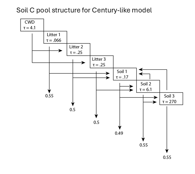
Figure 2.22.1 Pool structure, transitions, respired fractions (numbers at end of arrows), and turnover times (numbers in boxes) for the default, Century-based soil model in CLM.

The turnover times for the Century-based pool structure follow those described in Parton et al. (1988) (Table 2.22.1).

Table 2.22.1 Turnover times, C:N ratios, and acceleration parameters for the Century-based decomposition cascade.

	Turnover time (year)	C:N ratio	Acceleration term (\({a}_{i}\))
CWD	4.1		1
Litter 1	0.066		1
Litter 2	0.25		1
Litter 3	0.25		1
SOM 1	0.17	8	1
SOM 2	6.1	11	15
SOM 3	270	11	675

Likewise, values for the respiration fraction of Century-based structure are in Table 2.22.2.

Table 2.22.2 Respiration fractions for litter and SOM pools for Century-based structure

Pool	rf
\({rf}_{Lit1}\)	0.55
\({rf}_{Lit2}\)	0.5
\({rf}_{Lit3}\)	0.5
\({rf}_{SOM1}\)	f(txt)
\({rf}_{SOM2}\)	0.55
\({rf}_{SOM3}\)	0.55

2.22.2. Environmental modifiers on decomposition rate

These base rates are modified on each timestep by functions of the current soil environment. There are four rate modifiers: temperature (\({r}_{tsoil}\), unitless), moisture (\({r}_{water}\), unitless), an oxygen scalar (\({r}_{oxygen}\), unitless), and a depth scalar (\({r}_{depth}\), unitless).

The Temperature scalar \({r}_{tsoil}\) is calculated in CLM using a \({Q}_{10}\) approach, with \({Q}_{10} = 1.5\).

(2.22.1)\[r_{tsoil} =Q_{10} ^{\left(\frac{T_{soil,\, j} -T_{ref} }{10} \right)}\]

where j is the soil layer index, \({T}_{soil,j}\) (K) is the temperature of soil level j. The reference temperature \({T}_{ref}\) = 25C.

The rate scalar for soil water potential (\({r}_{water}\), unitless) is calculated using a relationship from Andrén and Paustian (1987) and supported by additional data in Orchard and Cook (1983):

(2.22.2)\[\begin{split}r_{water} =\sum _{j=1}^{5}\left\{\begin{array}{l} {0\qquad {\rm for\; }\Psi _{j} <\Psi _{\min } } \\ {\frac{\log \left({\Psi _{\min } \mathord{\left/ {\vphantom {\Psi _{\min } \Psi _{j} }} \right.} \Psi _{j} } \right)}{\log \left({\Psi _{\min } \mathord{\left/ {\vphantom {\Psi _{\min } \Psi _{\max } }} \right.} \Psi _{\max } } \right)} w_{soil,\, j} \qquad {\rm for\; }\Psi _{\min } \le \Psi _{j} \le \Psi _{\max } } \\ {1\qquad {\rm for\; }\Psi _{j} >\Psi _{\max } \qquad \qquad } \end{array}\right\}\end{split}\]

where \({\Psi}_{j}\) is the soil water potential in layer j, \({\Psi}_{min}\) is a lower limit for soil water potential control on decomposition rate. \({\Psi}_{max,j}\) (MPa) is the soil moisture at which decomposition proceeds at a moisture-unlimited rate. The default value of \({\Psi}_{max,j}\) for CLM6 is -0.002 MPa, nominally at field capacity. For frozen soils, the bulk of the rapid dropoff in decomposition with decreasing temperature is due to the moisture limitation, since matric potential is limited by temperature in the supercooled water formulation of Niu and Yang (2006),

(2.22.3)\[\psi \left(T\right)=-\frac{L_{f} \left(T-T_{f} \right)}{10^{3} T}\]

An additional frozen decomposition limitation can be specified using a 'frozen Q₁₀' following Koven et al. (2011), however the default value of this is the same as the unfrozen Q₁₀ value, and therefore the basic hypothesis is that frozen respiration is limited by liquid water availability, and can be modeled following the same approach as thawed but dry soils.

An additional rate scalar, \({r}_{oxygen}\) is enabled when the CH₄ submodel is used. This limits decomposition when there is insufficient molecular oxygen to satisfy stoichiometric demand (1 mol O₂ consumed per mol CO₂ produced) from heterotrophic decomposers, and supply from diffusion through soil layers (unsaturated and saturated) or aerenchyma (Chapter 2.26). A minimum value of \({r}_{oxygen}\) is set at 0.2, with the assumption that oxygen within organic tissues can supply the necessary stoichiometric demand at this rate. This value lies between estimates of 0.025–0.1 (Frolking et al. 2001), and 0.35 (Wania et al. 2009); the large range of these estimates poses a large unresolved uncertainty.

Lastly, a possible explicit depth dependence, \({r}_{depth}\), can be applied to soil C decomposition rates to account for processes other than temperature, moisture, and anoxia that can limit decomposition. This depth dependence of decomposition was shown by Jenkinson and Coleman (2008) to be an important term in fitting total C and 14C profiles, and implies that unresolved processes, such as priming effects, microscale anoxia, soil mineral surface and/or aggregate stabilization may be important in controlling the fate of carbon at depth Koven et al. (2013). CLM includes these unresolved depth controls via an exponential decrease in the soil turnover time with depth:

(2.22.4)\[r_{depth} =\exp \left(-\frac{z}{z_{\tau } } \right)\]

where \({z}_{\tau}\) is the e-folding depth for decomposition. For CLM6, the e-folding depth is 10m, which effectively means that intrinsic decomposition rates may proceed as quickly at depth as at the surface.

The combined decomposition rate scalar (\({r}_{total}\),unitless) is:

(2.22.5)\[r_{total} =r_{tsoil} r_{water} r_{oxygen} r_{depth} .\]

2.22.3. Management modifiers on decomposition rate

Tillage of cropland soil is represented as an additional rate scalar that depends on tillage intensity (default off), soil pool, and time since planting (Graham et al., 2021). The tillage enhancement is strongest in the first 14 days after planting (idpp < 15), weaker in the next 30 days (15 ≤ idpp < 45), weaker still in the next 30 days (45 ≤ idpp < 75), and nonexistent after that (idpp ≥ 75).

Table 2.22.3 Tillage decomposition rate scalars. Values in each cell represent enhancement in different periods of days past planting: [0, 14], [15, 44], [45, 74].

	low	high
Litter 2 (cel_lit)	1.5, 1.5, 1.1	1.8, 1.5, 1.1
Litter 3 (lig_lit)	1.5, 1.5, 1.1	1.8, 1.5, 1.1
SOM 1 (act_som)	1.0, 1.0, 1.0	1.2, 1.0, 1.0
SOM 2 (slo_som)	3.0, 1.6, 1.3	4.8, 3.5, 2.5
SOM 3 (pas_som)	3.0, 1.6, 1.3	4.8, 3.5, 2.5

2.22.4. N-limitation of Decomposition Fluxes

Decomposition rates can also be limited by the availability of mineral nitrogen, but calculation of this limitation depends on first estimating the potential rates of decomposition, assuming an unlimited mineral nitrogen supply. The general case is described here first, referring to a generic decomposition flux from an "upstream" pool (u) to a "downstream" pool (d), with an intervening loss due to respiration The potential carbon flux out of the upstream pool (\({CF}_{pot,u}\), gC m^-2 s^-1) is:

(2.22.6)\[CF_{pot,\, u} =CS_{u} k_{u}\]

where \({CS}_{u}\) (gC m^-2) is the initial mass in the upstream pool and \({k}_{u}\) is the decay rate constant (s^-1) for the upstream pool, adjusted for temperature and moisture conditions. Depending on the C:N ratios of the upstream and downstream pools and the amount of carbon lost in the transformation due to respiration (the respiration fraction), the execution of this potential carbon flux can generate either a source or a sink of new mineral nitrogen (\({NF}_{pot\_min,u}\)\({}_{\rightarrow}\)\({}_{d}\), gN m^-2 s^-1). The governing equation (Thornton and Rosenbloom, 2005) is:

(2.22.7)\[NF_{pot\_ min,\, u\to d} =\frac{CF_{pot,\, u} \left(1-rf_{u} -\frac{CN_{d} }{CN_{u} } \right)}{CN_{d} }\]

where \({rf}_{u}\) is the respiration fraction for fluxes leaving the upstream pool, \({CN}_{u}\) and \({CN}_{d}\) are the C:N ratios for upstream and downstream pools, respectively Negative values of \({NF}_{pot\_min,u}\)\({}_{\rightarrow}\)\({}_{d}\) indicate that the decomposition flux results in a source of new mineral nitrogen, while positive values indicate that the potential decomposition flux results in a sink (demand) for mineral nitrogen.

Following from the general case, potential carbon fluxes leaving individual pools in the decomposition cascade are given as:

(2.22.8)\[CF_{pot,\, Lit1} ={CS_{Lit1} k_{Lit1} r_{total} \mathord{\left/ {\vphantom {CS_{Lit1} k_{Lit1} r_{total} \Delta t}} \right.} \Delta t}\]

(2.22.9)\[CF_{pot,\, Lit2} ={CS_{Lit2} k_{Lit2} r_{total} \mathord{\left/ {\vphantom {CS_{Lit2} k_{Lit2} r_{total} \Delta t}} \right.} \Delta t}\]

(2.22.10)\[CF_{pot,\, Lit3} ={CS_{Lit3} k_{Lit3} r_{total} \mathord{\left/ {\vphantom {CS_{Lit3} k_{Lit3} r_{total} \Delta t}} \right.} \Delta t}\]

(2.22.11)\[CF_{pot,\, SOM1} ={CS_{SOM1} k_{SOM1} r_{total} \mathord{\left/ {\vphantom {CS_{SOM1} k_{SOM1} r_{total} \Delta t}} \right.} \Delta t}\]

(2.22.12)\[CF_{pot,\, SOM2} ={CS_{SOM2} k_{SOM2} r_{total} \mathord{\left/ {\vphantom {CS_{SOM2} k_{SOM2} r_{total} \Delta t}} \right.} \Delta t}\]

(2.22.13)\[CF_{pot,\, SOM3} ={CS_{SOM3} k_{SOM3} r_{total} \mathord{\left/ {\vphantom {CS_{SOM3} k_{SOM3} r_{total} \Delta t}} \right.} \Delta t}\]

where the factor (1/\(\Delta\)t) is included because the rate constant is calculated for the entire timestep (see equations above), but the convention is to express all fluxes on a per-second basis. Potential mineral nitrogen fluxes associated with these decomposition steps are:

(2.22.14)\[NF_{pot\_ min,\, Lit1\to SOM1} ={CF_{pot,\, Lit1} \left(1-rf_{Lit1} -\frac{CN_{SOM1} }{CN_{Lit1} } \right)\mathord{\left/ {\vphantom {CF_{pot,\, Lit1} \left(1-rf_{Lit1} -\frac{CN_{SOM1} }{CN_{Lit1} } \right) CN_{SOM1} }} \right.} CN_{SOM1} }\]

(2.22.15)\[NF_{pot\_ min,\, Lit2\to SOM1} ={CF_{pot,\, Lit2} \left(1-rf_{Lit2} -\frac{CN_{SOM1} }{CN_{Lit2} } \right)\mathord{\left/ {\vphantom {CF_{pot,\, Lit2} \left(1-rf_{Lit2} -\frac{CN_{SOM1} }{CN_{Lit2} } \right) CN_{SOM1} }} \right.} CN_{SOM1} }\]

(2.22.16)\[NF_{pot\_ min,\, Lit3\to SOM2} ={CF_{pot,\, Lit3} \left(1-rf_{Lit3} -\frac{CN_{SOM2} }{CN_{Lit3} } \right)\mathord{\left/ {\vphantom {CF_{pot,\, Lit3} \left(1-rf_{Lit3} -\frac{CN_{SOM2} }{CN_{Lit3} } \right) CN_{SOM2} }} \right.} CN_{SOM2} }\]

(2.22.17)\[NF_{pot\_ min,\, SOM1\to SOM2} ={CF_{pot,\, SOM1} \left(1-rf_{SOM1} -\frac{CN_{SOM2} }{CN_{SOM1} } \right)\mathord{\left/ {\vphantom {CF_{pot,\, SOM1} \left(1-rf_{SOM1} -\frac{CN_{SOM2} }{CN_{SOM1} } \right) CN_{SOM2} }} \right.} CN_{SOM2} }\]

(2.22.18)\[NF_{pot\_ min,\, SOM2\to SOM3} ={CF_{pot,\, SOM2} \left(1-rf_{SOM2} -\frac{CN_{SOM3} }{CN_{SOM2} } \right)\mathord{\left/ {\vphantom {CF_{pot,\, SOM2} \left(1-rf_{SOM2} -\frac{CN_{SOM3} }{CN_{SOM2} } \right) CN_{SOM3} }} \right.} CN_{SOM3} }\]

(2.22.19)\[NF_{pot\_ min,\, SOM1\to SOM3} ={CF_{pot,\, SOM1} \left(1-rf_{SOM1} -\frac{CN_{SOM3} }{CN_{SOM1} } \right)\mathord{\left/ {\vphantom {CF_{pot,\, SOM3} \left(1-rf_{SOM1} -\frac{CN_{SOM3} }{CN_{SOM1} } \right) CN_{SOM3} }} \right.} CN_{SOM3} }\]

(2.22.20)\[NF_{pot\_ min,\, SOM2\to SOM1} ={CF_{pot,\, SOM2} \left(1-rf_{SOM2} -\frac{CN_{SOM1} }{CN_{SOM2} } \right)\mathord{\left/ {\vphantom {CF_{pot,\, SOM1} \left(1-rf_{SOM2} -\frac{CN_{SOM1} }{CN_{SOM2} } \right) CN_{SOM1} }} \right.} CN_{SOM1} }\]

(2.22.21)\[NF_{pot\_ min,\, SOM3\to SOM1} ={CF_{pot,\, SOM3} \left(1-rf_{SOM3} -\frac{CN_{SOM1} }{CN_{SOM3} } \right)\mathord{\left/ {\vphantom {CF_{pot,\, SOM1} \left(1-rf_{SOM3} -\frac{CN_{SOM1} }{CN_{SOM3} } \right) CN_{SOM1} }} \right.} CN_{SOM1} }\]

Steps in the decomposition cascade that result in release of new mineral nitrogen (mineralization fluxes) are allowed to proceed at their potential rates, without modification for nitrogen availability. Steps that result in an uptake of mineral nitrogen (immobilization fluxes) are subject to rate limitation, depending on the availability of mineral nitrogen, the total immobilization demand, and the total demand for soil mineral nitrogen to support new plant growth. The potential mineral nitrogen fluxes from Eqs. (2.22.14)-(2.22.21) are evaluated, summing all the positive fluxes to generate the total potential nitrogen immobilization flux (\({NF}_{immob\_demand}\), gN m^-2 s^-1), and summing absolute values of all the negative fluxes to generate the total nitrogen mineralization flux (\({NF}_{gross\_nmin}\), gN m^-2 s^-1). Since \({NF}_{gross\_nmin}\) is a source of new mineral nitrogen to the soil mineral nitrogen pool it is not limited by the availability of soil mineral nitrogen, and is therefore an actual as opposed to a potential flux.

2.22.5. N Competition between plant uptake and soil immobilization fluxes

Once \({NF}_{immob\_demand }\) and \({NF}_{nit\_demand }\) for each layer j are known, the competition between plant and microbial nitrogen demand can be resolved. Mineral nitrogen in the soil pool (\({NS}_{sminn}\), gN m^-2) at the beginning of the timestep is considered the available supply.

Here, the \({NF}_{plant\_demand}\) is the theoretical maximum demand for nitrogen by plants to meet the entire carbon uptake given an N cost of zero (and therefore represents the upper bound on N requirements). N uptake costs that are \(>\) 0 imply that the plant will take up less N that it demands, ultimately. However, given the heuristic nature of the N competition algorithm, this discrepancy is not explicitly resolved here.

The hypothetical plant nitrogen demand from the soil mineral pool is distributed between layers in proportion to the profile of available mineral N:

(2.22.22)\[NF_{plant\_ demand,j} = NF_{plant\_ demand} NS_{sminn\_ j} / \sum _{j=1}^{nj}NS_{sminn,j}\]

Plants first compete for ammonia (NH4). For each soil layer (j), we calculate the total NH4 demand as:

(2.22.23)\[NF_{total\_ demand_nh4,j} = NF_{immob\_ demand,j} + NF_{immob\_ demand,j} + NF_{nit\_ demand,j}\]

where If \({NF}_{total\_demand,j}\)\(\Delta\)t \(<\) \({NS}_{sminn,j}\), then the available pool is large enough to meet both the maximum plant and microbial demand, then immobilization proceeds at the maximum rate.

(2.22.24)\[f_{immob\_demand,j} = 1.0\]

where \({f}_{immob\_demand,j}\) is the fraction of potential immobilization demand that can be met given current supply of mineral nitrogen in this layer. We also set the actual nitrification flux to be the same as the potential flux (\(NF_{nit}\) = \(NF_{nit\_ demand}\)).

If \({NF}_{total\_demand,j} \Delta t \mathrm{\ge} {NS}_{sminn,j}\), then there is not enough mineral nitrogen to meet the combined demands for plant growth and heterotrophic immobilization, immobilization is reduced proportional to the discrepancy, by \(f_{immob\_ demand,j}\), where

(2.22.25)\[f_{immob\_ demand,j} = \frac{NS_{sminn,j} }{\Delta t\, NF_{total\_ demand,j} }\]

The N available to the FUN model for plant uptake (\({NF}_ {plant\_ avail\_ sminn}\) (gN m^-2), which determines both the cost of N uptake, and the absolute limit on the N which is available for acquisition, is calculated as the total mineralized pool minus the actual immobilized flux:

(2.22.26)\[NF_{plant\_ avail\_ sminn,j} = NS_{sminn,j} - f_{immob\_demand} NF_{immob\_ demand,j}\]

This treatment of competition for nitrogen as a limiting resource is referred to a demand-based competition, where the fraction of the available resource that eventually flows to a particular process depends on the demand from that process in comparison to the total demand from all processes. Processes expressing a greater demand acquire a larger vfraction of the available resource.

2.22.6. Final Decomposition Fluxes

With \({f}_{immob\_demand}\) known, final decomposition fluxes can be calculated. Actual carbon fluxes leaving the individual litter and SOM pools are calculated as:

(2.22.27)\[\begin{split}CF_{Lit1} =\left\{\begin{array}{l} {CF_{pot,\, Lit1} f_{immob\_ demand} \qquad {\rm for\; }NF_{pot\_ min,\, Lit1\to SOM1} >0} \\ {CF_{pot,\, Lit1} \qquad {\rm for\; }NF_{pot\_ min,\, Lit1\to SOM1} \le 0} \end{array}\right\}\end{split}\]

(2.22.28)\[\begin{split}CF_{Lit2} =\left\{\begin{array}{l} {CF_{pot,\, Lit2} f_{immob\_ demand} \qquad {\rm for\; }NF_{pot\_ min,\, Lit2\to SOM1} >0} \\ {CF_{pot,\, Lit2} \qquad {\rm for\; }NF_{pot\_ min,\, Lit2\to SOM1} \le 0} \end{array}\right\}\end{split}\]

(2.22.29)\[\begin{split}CF_{Lit3} =\left\{\begin{array}{l} {CF_{pot,\, Lit3} f_{immob\_ demand} \qquad {\rm for\; }NF_{pot\_ min,\, Lit3\to SOM2} >0} \\ {CF_{pot,\, Lit3} \qquad {\rm for\; }NF_{pot\_ min,\, Lit3\to SOM2} \le 0} \end{array}\right\}\end{split}\]

(2.22.30)\[\begin{split}CF_{SOM1} =\left\{\begin{array}{l} {CF_{pot,\, SOM1} f_{immob\_ demand} \qquad {\rm for\; }NF_{pot\_ min,\, SOM1\to SOM2} >0} \\ {CF_{pot,\, SOM1} \qquad {\rm for\; }NF_{pot\_ min,\, SOM1\to SOM2} \le 0} \end{array}\right\}\end{split}\]

(2.22.31)\[\begin{split}CF_{SOM2} =\left\{\begin{array}{l} {CF_{pot,\, SOM2} f_{immob\_ demand} \qquad {\rm for\; }NF_{pot\_ min,\, SOM2\to SOM3} >0} \\ {CF_{pot,\, SOM2} \qquad {\rm for\; }NF_{pot\_ min,\, SOM2\to SOM3} \le 0} \end{array}\right\}\end{split}\]

(2.22.32)\[\begin{split}CF_{SOM1} =\left\{\begin{array}{l} {CF_{pot,\, SOM1} f_{immob\_ demand} \qquad {\rm for\; }NF_{pot\_ min,\, SOM1\to SOM3} >0} \\ {CF_{pot,\, SOM1} \qquad {\rm for\; }NF_{pot\_ min,\, SOM1\to SOM3} \le 0} \end{array}\right\}\end{split}\]

(2.22.33)\[\begin{split}CF_{SOM2} =\left\{\begin{array}{l} {CF_{pot,\, SOM2} f_{immob\_ demand} \qquad {\rm for\; }NF_{pot\_ min,\, SOM2\to SOM1} >0} \\ {CF_{pot,\, SOM2} \qquad {\rm for\; }NF_{pot\_ min,\, SOM2\to SOM1} \le 0} \end{array}\right\}\end{split}\]

(2.22.34)\[\begin{split}CF_{SOM3} =\left\{\begin{array}{l} {CF_{pot,\, SOM3} f_{immob\_ demand} \qquad {\rm for\; }NF_{pot\_ min,\, SOM3\to SOM1} >0} \\ {CF_{pot,\, SOM3} \qquad {\rm for\; }NF_{pot\_ min,\, SOM3\to SOM1} \le 0} \end{array}\right\}\end{split}\]

Heterotrophic respiration fluxes (losses of carbon as CO₂ to the atmosphere) are:

(2.22.35)\[CF_{Lit1,\, HR} =CF_{Lit1} rf_{Lit1}\]

(2.22.36)\[CF_{Lit2,\, HR} =CF_{Lit2} rf_{Lit2}\]

(2.22.37)\[CF_{Lit3,\, HR} =CF_{Lit3} rf_{Lit3}\]

(2.22.38)\[CF_{SOM1,\, HR} =CF_{SOM1} rf_{SOM1}\]

(2.22.39)\[CF_{SOM2,\, HR} =CF_{SOM2} rf_{SOM2}\]

(2.22.40)\[CF_{SOM3,\, HR} =CF_{SOM3} rf_{SOM3}\]

Transfers of carbon from upstream to downstream pools in the decomposition cascade are given as:

(2.22.41)\[CF_{Lit1,\, SOM1} =CF_{Lit1} \left(1-rf_{Lit1} \right)\]

(2.22.42)\[CF_{Lit2,\, SOM1} =CF_{Lit2} \left(1-rf_{Lit2} \right)\]

(2.22.43)\[CF_{Lit3,\, SOM2} =CF_{Lit3} \left(1-rf_{Lit3} \right)\]

(2.22.44)\[CF_{SOM1,\, SOM2} =CF_{SOM1} \left(1-rf_{SOM1} \right)\]

(2.22.45)\[CF_{SOM2,\, SOM3} =CF_{SOM2} \left(1-rf_{SOM2} \right)\]

(2.22.46)\[CF_{SOM1,\, SOM3} =CF_{SOM1} \left(1-rf_{SOM1} \right)\]

(2.22.47)\[CF_{SOM2,\, SOM1} =CF_{SOM2} \left(1-rf_{SOM2} \right)\]

(2.22.48)\[CF_{SOM3,\, SOM1} =CF_{SOM3} \left(1-rf_{SOM3} \right)\]

In accounting for the fluxes of nitrogen between pools in the decomposition cascade and associated fluxes to or from the soil mineral nitrogen pool, the model first calculates a flux of nitrogen from an upstream pool to a downstream pool, then calculates a flux either from the soil mineral nitrogen pool to the downstream pool (immobilization or from the downstream pool to the soil mineral nitrogen pool (mineralization). Transfers of nitrogen from upstream to downstream pools in the decomposition cascade are given as:

(2.22.49)\[NF_{Lit1,\, SOM1} ={CF_{Lit1} \mathord{\left/ {\vphantom {CF_{Lit1} CN_{Lit1} }} \right.} CN_{Lit1} }\]

(2.22.50)\[NF_{Lit2,\, SOM1} ={CF_{Lit2} \mathord{\left/ {\vphantom {CF_{Lit2} CN_{Lit2} }} \right.} CN_{Lit2} }\]

(2.22.51)\[NF_{Lit3,\, SOM2} ={CF_{Lit3} \mathord{\left/ {\vphantom {CF_{Lit3} CN_{Lit3} }} \right.} CN_{Lit3} }\]

(2.22.52)\[NF_{SOM1,\, SOM2} ={CF_{SOM1} \mathord{\left/ {\vphantom {CF_{SOM1} CN_{SOM1} }} \right.} CN_{SOM1} }\]

(2.22.53)\[NF_{SOM2,\, SOM3} ={CF_{SOM2} \mathord{\left/ {\vphantom {CF_{SOM2} CN_{SOM2} }} \right.} CN_{SOM2} }\]

(2.22.54)\[NF_{SOM1,\, SOM3} ={CF_{SOM1} \mathord{\left/ {\vphantom {CF_{SOM1} CN_{SOM1} }} \right.} CN_{SOM1} }\]

(2.22.55)\[NF_{SOM2,\, SOM1} ={CF_{SOM2} \mathord{\left/ {\vphantom {CF_{SOM2} CN_{SOM2} }} \right.} CN_{SOM2} }\]

(2.22.56)\[NF_{SOM3,\, SOM1} ={CF_{SOM3} \mathord{\left/ {\vphantom {CF_{SOM3} CN_{SOM3} }} \right.} CN_{SOM3} }\]

Corresponding fluxes to or from the soil mineral nitrogen pool depend on whether the decomposition step is an immobilization flux or a mineralization flux:

(2.22.57)\[\begin{split}NF_{sminn,\, Lit1\to SOM1} =\left\{\begin{array}{l} {NF_{pot\_ min,\, Lit1\to SOM1} f_{immob\_ demand} \qquad {\rm for\; }NF_{pot\_ min,\, Lit1\to SOM1} >0} \\ {NF_{pot\_ min,\, Lit1\to SOM1} \qquad {\rm for\; }NF_{pot\_ min,\, Lit1\to SOM1} \le 0} \end{array}\right\}\end{split}\]

(2.22.58)\[\begin{split}NF_{sminn,\, Lit2\to SOM1} =\left\{\begin{array}{l} {NF_{pot\_ min,\, Lit2\to SOM1} f_{immob\_ demand} \qquad {\rm for\; }NF_{pot\_ min,\, Lit2\to SOM1} >0} \\ {NF_{pot\_ min,\, Lit2\to SOM1} \qquad {\rm for\; }NF_{pot\_ min,\, Lit2\to SOM1} \le 0} \end{array}\right\}\end{split}\]

(2.22.59)\[\begin{split}NF_{sminn,\, Lit3\to SOM2} =\left\{\begin{array}{l} {NF_{pot\_ min,\, Lit3\to SOM2} f_{immob\_ demand} \qquad {\rm for\; }NF_{pot\_ min,\, Lit3\to SOM2} >0} \\ {NF_{pot\_ min,\, Lit3\to SOM2} \qquad {\rm for\; }NF_{pot\_ min,\, Lit3\to SOM2} \le 0} \end{array}\right\}\end{split}\]

(2.22.60)\[\begin{split}NF_{sminn,SOM1\to SOM2} =\left\{\begin{array}{l} {NF_{pot\_ min,\, SOM1\to SOM2} f_{immob\_ demand} \qquad {\rm for\; }NF_{pot\_ min,\, SOM1\to SOM2} >0} \\ {NF_{pot\_ min,\, SOM1\to SOM2} \qquad {\rm for\; }NF_{pot\_ min,\, SOM1\to SOM2} \le 0} \end{array}\right\}\end{split}\]

(2.22.61)\[\begin{split}NF_{sminn,SOM2\to SOM3} =\left\{\begin{array}{l} {NF_{pot\_ min,\, SOM2\to SOM3} f_{immob\_ demand} \qquad {\rm for\; }NF_{pot\_ min,\, SOM2\to SOM3} >0} \\ {NF_{pot\_ min,\, SOM2\to SOM3} \qquad {\rm for\; }NF_{pot\_ min,\, SOM2\to SOM3} \le 0} \end{array}\right\}\end{split}\]

(2.22.62)\[\begin{split}NF_{sminn,SOM1\to SOM3} =\left\{\begin{array}{l} {NF_{pot\_ min,\, SOM1\to SOM3} f_{immob\_ demand} \qquad {\rm for\; }NF_{pot\_ min,\, SOM1\to SOM3} >0} \\ {NF_{pot\_ min,\, SOM1\to SOM3} \qquad {\rm for\; }NF_{pot\_ min,\, SOM1\to SOM3} \le 0} \end{array}\right\}\end{split}\]

(2.22.63)\[\begin{split}NF_{sminn,SOM2\to SOM1} =\left\{\begin{array}{l} {NF_{pot\_ min,\, SOM2\to SOM1} f_{immob\_ demand} \qquad {\rm for\; }NF_{pot\_ min,\, SOM2\to SOM1} >0} \\ {NF_{pot\_ min,\, SOM2\to SOM1} \qquad {\rm for\; }NF_{pot\_ min,\, SOM2\to SOM1} \le 0} \end{array}\right\}\end{split}\]

(2.22.64)\[\begin{split}NF_{sminn,SOM3\to SOM1} =\left\{\begin{array}{l} {NF_{pot\_ min,\, SOM3\to SOM1} f_{immob\_ demand} \qquad {\rm for\; }NF_{pot\_ min,\, SOM3\to SOM1} >0} \\ {NF_{pot\_ min,\, SOM3\to SOM1} \qquad {\rm for\; }NF_{pot\_ min,\, SOM3\to SOM1} \le 0} \end{array}\right\}\end{split}\]

2.22.7. Vertical Distribution and Transport of Decomposing C and N pools

Additional terms are needed to calculate the vertically-resolved soil C and N budget: the initial vertical distribution of C and N from PFTs delivered to the litter and CWD pools, and the vertical transport of C and N pools.

For initial vertical inputs, CLM uses separate profiles for aboveground (leaf, stem) and belowground (root) inputs. Aboveground inputs are given a single exponential with default e-folding depth = 0.1m. Belowground inputs are distributed according to rooting profiles with default values based on the Jackson et al. (1996) exponential parameterization.

Vertical mixing is accomplished by an advection-diffusion equation. The goal of this is to consider slow, soild- and adsorbed-phase transport due to bioturbation, cryoturbation, and erosion. Faster aqueous-phase transport is not included in CLM, but has been developed as part of the CLM-BeTR suite of parameterizations (Tang and Riley 2013). The default value of the advection term is 0 cm/yr, such that transport is purely diffusive. Diffusive transport differs in rate between permafrost soils (where cryoturbation is the dominant transport term) and non-permafrost soils (where bioturbation dominates). For permafrost soils, a parameterization based on that of Koven et al. (2009) is used: the diffusivity parameter is constant through the active layer, and decreases linearly from the base of the active layer to zero at a set depth (default 3m); the default permafrost diffusivity is 5 cm²/yr. For non-permafrost soils, the default diffusivity is 1 cm²/yr.

2.22.8. Model Equilibration and its Acceleration

For transient experiments, it is usually assumed that the carbon cycle is starting from a point of relatively close equilibrium, i.e. that productivity is balanced by ecosystem carbon losses through respiratory and disturbance pathways. In order to satisfy this assumption, the model is generally run until the productivity and loss terms find a stable long-term equilibrium; at this point the model is considered 'spun up'.

Because of the coupling between the slowest SOM pools and productivity through N downregulation of photosynthesis, equilibration of the model for initialization purposes will take an extremely long time in the standard mode. This is particularly true for the CENTURY-based decomposition cascade, which includes a passive pool. In order to rapidly equilibrate the model, a modified version of the "accelerated decomposition" (Thornton and Rosenbloon, 2005) is used. The fundamental idea of this approach is to allow fluxes between the various pools (both turnover-defined and vertically-defined fluxes) adjust rapidly, while keeping the pool sizes themselves small so that they can fill quickly To do this, the base decomposition rate \({k}_{i}\) for each pool i is accelerated by a term \({a}_{i}\) such that the slow pools are collapsed onto an approximately annual timescale Koven et al. (2013). Accelerating the pools beyond this timescale distorts the seasonal and/or diurnal cycles of decomposition and N mineralization, thus leading to a substantially different ecosystem productivity than the full model. For the vertical model, the vertical transport terms are also accelerated by the same term \({a}_{i}\), as is the radioactive decay when \({}^{14}\)C is enabled, following the same principle of keeping fluxes between pools (or fluxes lost to decay close to the full model while keeping the pools sizes small. When leaving the accelerated decomposition mode, the concentration of C and N in pools that had been accelerated are multiplied by the same term \({a}_{i}\), to bring the model into approximate equilibrium Note that in CLM, the model can also transition into accelerated decomposition mode from the standard mode (by dividing the pools by \({a}_{i}\)), and that the transitions into and out of accelerated decomposition mode are handled automatically by CLM upon loading from restart files (which preserve information about the mode of the model when restart files were written).

The base acceleration terms for the two decomposition cascades are shown in Table 2.22.1. In addition to the base terms, CLM5 also includes a geographic term to the acceleration in order to apply larger values to high-latitude systems, where decomposition rates are particularly slow and thus equilibration can take significantly longer than in temperate or tropical climates. This geographic term takes the form of a logistic equation, where \({a}_{i}\) is equal to the product of the base acceleration term and \({a}_{l}\) below:

(2.22.65)\[ a_l = 1 + 50 / \left ( 1 + exp \left (-0.1 * (abs(latitude) - 60 ) \right ) \right )\]

2.22.9. Alternate soil sub-model: MIMICS

In CLM6, there is a new capability to use the MIcrobial-MIneral Carbon Stabilization (MIMICS) model (Wieder et al. 2014; Wieder et al. 2015b; Kyker-Snowman et al. 2020) instead of the Century-like soil model. MIMICS is a microbially-explicit soil biogeochemical model that represents modern understanding about plant and microbial contributions to soil organic matter and mineral stabilization as a protection mechanism for soil organic matter. MIMICS has two litter pools, two microbial pools, and three soil organic matter pools that are connected as in Figure 2.22.2. Details about MIMICS-CN can be found in Kyker-Snowman et al. (2020).

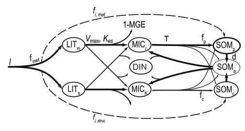
Figure 2.22.2 Wiring diagram for MIMICS soil submodel.

Unlike the Century-like soil model, MIMICS does not use first-order decomposition rates, and as such, has different parameters. MIMICS uses Michaelis-Menten kinetics which are governed by a max decomposition rate (Vmax) and half saturation constant (Km). The carbon flux is further modified by the carbon use efficiency (CUE), which is comparable to the respiration fraction in the default soil submodel. Vmax, Km, and CUE vary for each flux between microbial (MICr, MICk) and substrate pools (LITs, LITm, and SOMa). Both litter and microbial pools can contribute to the physically- and chemically-protected SOM (SOMp and SOMc), with those pools subsequently contributing to the available SOM pool (SOMa), which can be taken up by microbes. Coupling of C and N occurs in the microbial pools in MIMICS, where incoming C and N fluxes are summed and then adjusted by CUE and nitrogen use efficiency (default value = 0.85). If the C:N of the incoming substrates is greater than those of the microbial groups, overflow respiration (and consequently N immobilization) occurs. If the C:N of incoming substrates is less than those of the microbial groups, N mineralization occurs.

Because MIMICS uses different decomposition than the Century-like model, it requires a longer spin-up time. Currently, MIMICS is being spun up with an Anderson Acceleration method (Khatiwala, 2024).