2.16. Urban Model (CLMU)
The urban parameterization (CLMU; Oleson et al. (2008b); Oleson et al. (2008c); Oleson and Feddema (2020)) allows simulation of the urban environment within a climate model, and particularly the temperature/humidity where people live. As such, the urban model allows scientific study of how climate change affects the urban heat island and possible urban planning and design strategies to mitigate warming (e.g., white roofs).
Urban areas in CLM are represented by up to three urban landunits per gridcell according to density class. The urban landunit is based on the "urban canyon" concept of Oke (1987) in which the canyon geometry is described by building height (\(H\)) and street width (\(W\)) (Figure 2.16.1). The canyon system consists of roofs, walls, and canyon floor. Walls are further divided into shaded and sunlit components. The canyon floor is divided into pervious (e.g., to represent residential lawns, parks) and impervious (e.g., to represent roads, parking lots, sidewalks) fractions. Vegetation is not explicitly modeled for the pervious fraction; instead evaporation is parameterized by a simplified bulk scheme.
Each of the five urban surfaces is treated as a column within the landunit (Figure 2.16.1). Radiation parameterizations account for trapping of solar and longwave radiation inside the canyon. Momentum fluxes are determined for the urban landunit using a roughness length and displacement height appropriate for the urban canyon and stability formulations adopted from CLM. A one-dimensional heat conduction equation is solved numerically for a multiple-layer (\(N_{levurb} =10\)) column to determine conduction fluxes into and out of canyon surfaces.
Turbulent [sensible heat (\(Q_{H,\, u}\) ) and latent heat (\(Q_{E,\, u}\) )] and storage (\(Q_{S,\, u}\) ) heat fluxes and surface (\(T_{u,\, s}\) ) and internal (\(T_{u,\, i=1,\, N_{levgrnd} }\) ) temperatures are determined for each urban surface \(u\). Hydrology on the roof and canyon floor is simulated and walls are hydrologically inactive. A snowpack can form on the active surfaces. A certain amount of liquid water is allowed to pond on these surfaces which supports evaporation. Water in excess of the maximum ponding depth runs off (\(R_{roof},\, R_{imprvrd},\, R_{prvrd}\) ).
The heat and moisture fluxes from each surface interact with each other through a bulk air mass that represents air in the urban canopy layer for which specific humidity (\(q_{ac}\) ) and temperature (\(T_{ac}\) ) are prognosed (Figure 2.16.2). The air temperature can be compared with that from surrounding vegetated/soil (rural) surfaces in the model to ascertain heat island characteristics. As with other landunits, the CLMU is forced either with output from a host atmospheric model (e.g., the Community Atmosphere Model (CAM)) or observed forcing (e.g., reanalysis or field observations). The urban model produces sensible, latent heat, and momentum fluxes, emitted longwave, and reflected solar radiation, which are area-averaged with fluxes from non-urban "landunits" (e.g., vegetation, lakes) to supply grid cell averaged fluxes to the atmospheric model.
The version of the urban model that was first released as a component of CLM4.0 is separately described in the urban technical note (Oleson et al. (2010b)). The main changes in the urban model from CLM4.0 to CLM4.5 were 1) an expansion of the single urban landunit to up to three landunits per grid cell stratified by urban density types, 2) the number of urban layers for roofs and walls was no longer constrained to be equal to the number of ground layers, 3) space heating and air conditioning (AC) wasteheat factors were set to zero by default so that the user could customize these factors for their own application, 4) the elevation threshold used to eliminate urban areas in the surface dataset creation routines was increased from 2200 meters to 2600 meters, 5) hydrologic and thermal calculations for the pervious road followed CLM4.5 parameterizations.
The main changes in the urban model from CLM4.5 to CLM5.0 were 1) a more sophisticated and realistic building space heating and AC submodel (described below) that prognoses interior building air temperature and includes more realistic space heating and AC wasteheat factors (see above), 2) the maximum building temperature (which determines AC demand) was now read in from a file specified from the urbantv_streams namelist group instead of the surface dataset which allowed for dynamic control of this input variable. The maximum building temperatures that were defined in Jackson et al. (2010) are only implemented beginning in year 1950 (thus AC is off in prior years) and AC is turned off in year 2100 (because the buildings are not suitable for AC in some extreme global warming scenarios), 3) the inclusion of an optional updated urban properties dataset and new scenario tool. These features are described in more detail in Oleson and Feddema (2020). In addition, a module of heat stress indices calculated online in the model that can be used to assess human thermal comfort for rural and urban areas was added. This last development is described and evaluated by Buzan et al. (2015).
The main changes in the urban model from CLM5.0 to CLM6.0 are (see below) 1) an explicit AC scheme for the building energy model (BEM) that better captures AC energy flux, 2) the addition of transient urban capability (annual changes in urban fraction over the course of a simulation), 3) a slightly modified set of urban properties that were an option in CLM5.0 and are now used by default, 4) new datasets of urban extent (urban fraction of the grid cell) for 1700-2023 (2024- data expected soon also) based on CMIP7 LUH3 data.
The building energy model introduced in Oleson and Feddema (2020) accounts for the conduction of heat through interior surfaces (roof, sunlit and shaded walls, and floors), convection (sensible heat exchange) between interior surfaces and building air, longwave radiation exchange between interior surfaces, and ventilation (natural infiltration and exfiltration). Idealized HAC systems are assumed where the system capacity is infinite and the system supplies the amount of energy needed to keep the indoor air temperature (\(T_{iB}\)) within maximum and minimum emperatures (\(T_{iB,\, \max },\, T_{iB,\, \min }\) ), thus explicitly resolving space heating and AC fluxes. Anthropogenic sources of waste heat (\(Q_{H,\, waste}\) ) from HAC that account for inefficiencies in the heating and AC equipment and from energy lost in the conversion of primary energy sources to end use energy are derived from Sivak (2013). These sources of waste heat are incorporated as modifications to the canyon energy budget.
An explicit AC adoption parameterization for the BEM was developed for CLM6.0 (Li et al. (2024)). An AC adoption parameter is introduced (\(p_{AC}\) ). The AC flux is first calculated under saturated AC adoption (i.e., \(p_{AC}=100%\) ). The actual AC flux removed from the indoor air is then scaled based on \(p_{AC}\) and the waste heat added to the urban canyon due to AC energy use is also scaled by \(p_{AC}\). A global, spatially explicit dataset for the AC adoption rate was developed at country- and sub-country-level from sources such as the International Energy Agency (IEA), national surveys, scientific literature, and others. For use with CLM, the AC adoption parameter was regridded to 0.9° latitude by 1.25° longitude and is read in for each of the three urban density classes using the file specified by the urbantv_streams namelist group (variables p_ac_MD, p_ac_HD, p_ac_TBD). The maximum building interior temperature is also specified by the file in the urbantv_streams namelist group and is now considered to be the AC proxy setpoint in the parameterization and is set to 300K for all urban density classes (variables tbuildmax_MD', tbuildmax_HD, tbuildmax_TBD). The explicit AC adoption parameterization in combination with the AC adoption rate dataset significantly improve CLM's performance in model building AC energy flux, both in magnitude and spatial variability (Li et al. (2024)).
Global urban properties were originally developed by Jackson et al. (2010). For each of 33 distinct regions across the globe and four urban density classes [tall building district (TBD), and high, medium, and low density (HD, MD, LD)], thermal (e.g., heat capacity and thermal conductivity), radiative (e.g., albedo and emissivity) and morphological (e.g., height to width ratio, roof fraction, average building height, and pervious fraction of the canyon floor) properties, are provided for each of the density classes. Building interior minimum and maximum temperatures are prescribed based on climate and socioeconomic considerations. As described in Oleson and Feddema (2020) the urban properties dataset in Jackson et al. (2010) was modified with respect to wall and roof thermal properties to correct for biases in heat transfer due to layer and building type averaging. Further changes to the dataset reflect the need for scenario development, thus allowing for the creation of hypothetical wall types, and the easier interchange of wall facets. This slightly modified dataset was an option in CLM5.0.
The "raw" urban properties dataset used by the model is created from the urban properties tool which is available as part of the Toolbox for Human-Earth System Integration & Scaling (THESIS) tool set (https://github.com/NCAR/THESISUrbanPropertiesTool; Oleson and Feddema (2020)). The driver script (urban_prop.csh) specifies three input csv files (by default, mat_prop.csv, lam_spec.csv, and city_spec.csv; (Figure 2.16.3)) that describe the morphological, radiative, and thermal properties of urban areas, plus the minimum building interior temperature, and generates a global dataset at 0.05° latitude by longitude in NetCDF format. This dataset, when combined with the urban extent data described below, is then ingested into the mksurfdata_esmf tool to create surface datasets at the desired spatial and temporal resolutions.
Urban extent (circa-year 2000), defined for the four density classes, was originally provided by Jackson et al. (2010) and derived from LandScan 2004, a population density dataset derived from census data, nighttime lights satellite observations, road proximity, and slope (Dobson et al. 2000). Note that the LD class is not used in CLM because it is highly rural (dominated by vegetation) and better modeled as a vegetated/soil surface. This dataset was used for model versions CLM5.0 and earlier. A more up to date urban extent dataset was derived for use with CLM6.0 from a 0.05° urban landcover projection dataset (Gao and O'Neill (2020)) as described in Fang et al. (2026) (code and auxiliary datasets available at https://figshare.com/s/4a890655b34498c1d082). The Gao and O'Neill (2020) dataset provides global urban land cover for 2000-2100 in decadal intervals for a historical baseline (year 2000) and five CMIP6 ScenarioMIP Shared Socioeconomic Pathways (SSPs) at 0.05° resolution (2010-2100). Briefly, because the Gao and O'Neill (2020) dataset only provides the data as a single urban class, the urban area in each grid cell is partitioned according to the ratio of the density types in that grid cell in the Jackson et al. (2010) dataset. The decadal urban data are then linearly interpolated to generate annual urban data from 2015-2100. To provide data prior to 2015, the average urban fraction of the five SSP scenarios was calculated in 2010 and 2015. Then annual urban fraction from 2000 to 2014 were obtained by interpolating betwen urban fraction in the historical baseline year 2000, and average SSP years 2010 and 2015. Finally, due to a lack of historical data, data for 1850-1999 were simply copied from year 2000 data. The yearly Gao and O'Neill (2020) historical and SSP datasets are available for an intermediate model version (CTSM5.3) at 0.05° resolution.
However, it was deemed desirable to create a dataset consistent with CMIP7 landcover change protocols. CMIP7 provides urban fraction at 0.25° resolution for 1700-2023. Again, since the dataset only provides the data as a single urban class, the urban area in each grid cell is partitioned according to the ratio of the density types in that grid cell in a year 2023 0.25° resolution version of the Gao and O'Neill (2020) dataset created as described above. An exception is that the TBD class is not allowed before year 1900 as skyscrapers, etc. had not yet begun to be built. In that case, the urban fraction was split proportionally between the HD and MD classes. Datasets for future scenarios, i.e., 2024-, will be created similarly when CMIP7 data is available.
To accomodate the transient urban datasets developed above, dynamic urban capability was implemented into the model as described in Fang et al. (2026) in a manner similar to the implementation of other land cover transient datasets including ensuring conservation for total gridcell water and energy content. See Chapter 2.28 for further details.

Figure 2.16.1 Schematic representation of the urban land unit. See the text for description of notation. Incident, reflected, and net solar and longwave radiation are calculated for each individual surface but are not shown for clarity.
Figure 2.16.2 Schematic of urban and atmospheric model coupling. The urban model is forced by the atmospheric model wind (\(u_{atm}\) ), temperature (\(T_{atm}\) ), specific humidity (\(q_{atm}\) ), precipitation (\(P_{atm}\) ), solar (\(S_{atm} \, \downarrow\) ) and longwave (\(L_{atm} \, \downarrow\) ) radiation at reference height \(z'_{atm}\) (section 2.2.3.1). Fluxes from the urban landunit to the atmosphere are turbulent sensible (\(H\)) and latent heat (\(\lambda E\)), momentum (\(\tau\) ), albedo (\(I\uparrow\) ), emitted longwave (\(L\uparrow\) ), and absorbed shortwave (\(\vec{S}\)) radiation. Air temperature (\(T_{ac}\) ), specific humidity (\(q_{ac}\) ), and wind speed (\(u_{c}\) ) within the urban canopy layer are diagnosed by the urban model. \(H\) is the average building height.
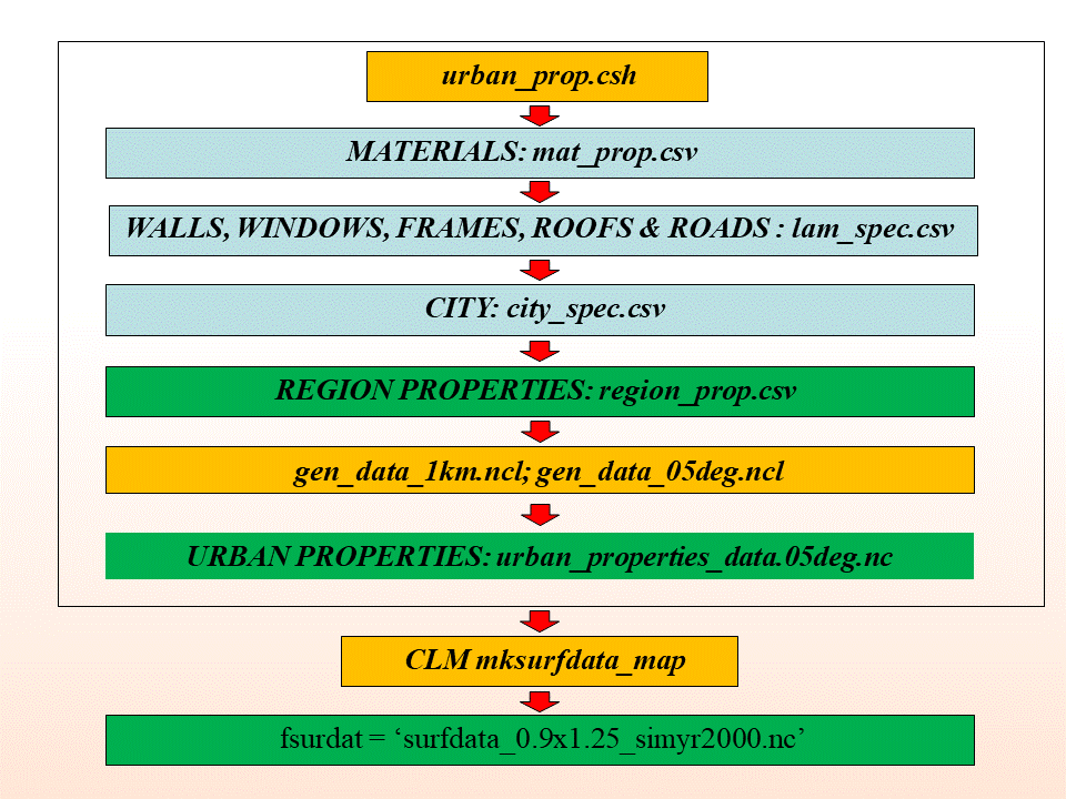
Figure 2.16.3 Schematic of THESIS urban properties tool. Executable scripts are in orange, input files are blue, and output files are green. Items within the black box outline are either read in as input, executed, or output by the driver script (urban_prop.csh).